Arrays: Memory Layout & Applications

Arrays are one of the most fundamental data structures in computer science. Nearly every complex data structure — such as matrices, heaps, hash tables, and graphs — builds upon arrays.

An array stores multiple elements of the same type in contiguous memory locations, allowing efficient access and manipulation of data.

Because of their simplicity and efficiency, arrays are widely used in:

• Operating systems
• Databases
• Graphics processing
• Scientific computing
• Machine learning
• Competitive programming

This article explores the memory layout of arrays, how indexing works, and their practical applications.

What is an Array?

An array is a collection of elements stored in continuous memory locations.

Each element can be accessed using an index.

Example

Array A = [10, 20, 30, 40, 50]

Index	Value
0	10
1	20
2	30
3	40
4	50

Most programming languages use zero-based indexing.

Python Example

# creating an array (Python list)
A = [10, 20, 30, 40, 50]

# accessing elements
print(A[0])   # Output: 10
print(A[2])   # Output: 30
print(A[4])   # Output: 50

Accessing any element takes O(1) time.

Memory Layout of Arrays

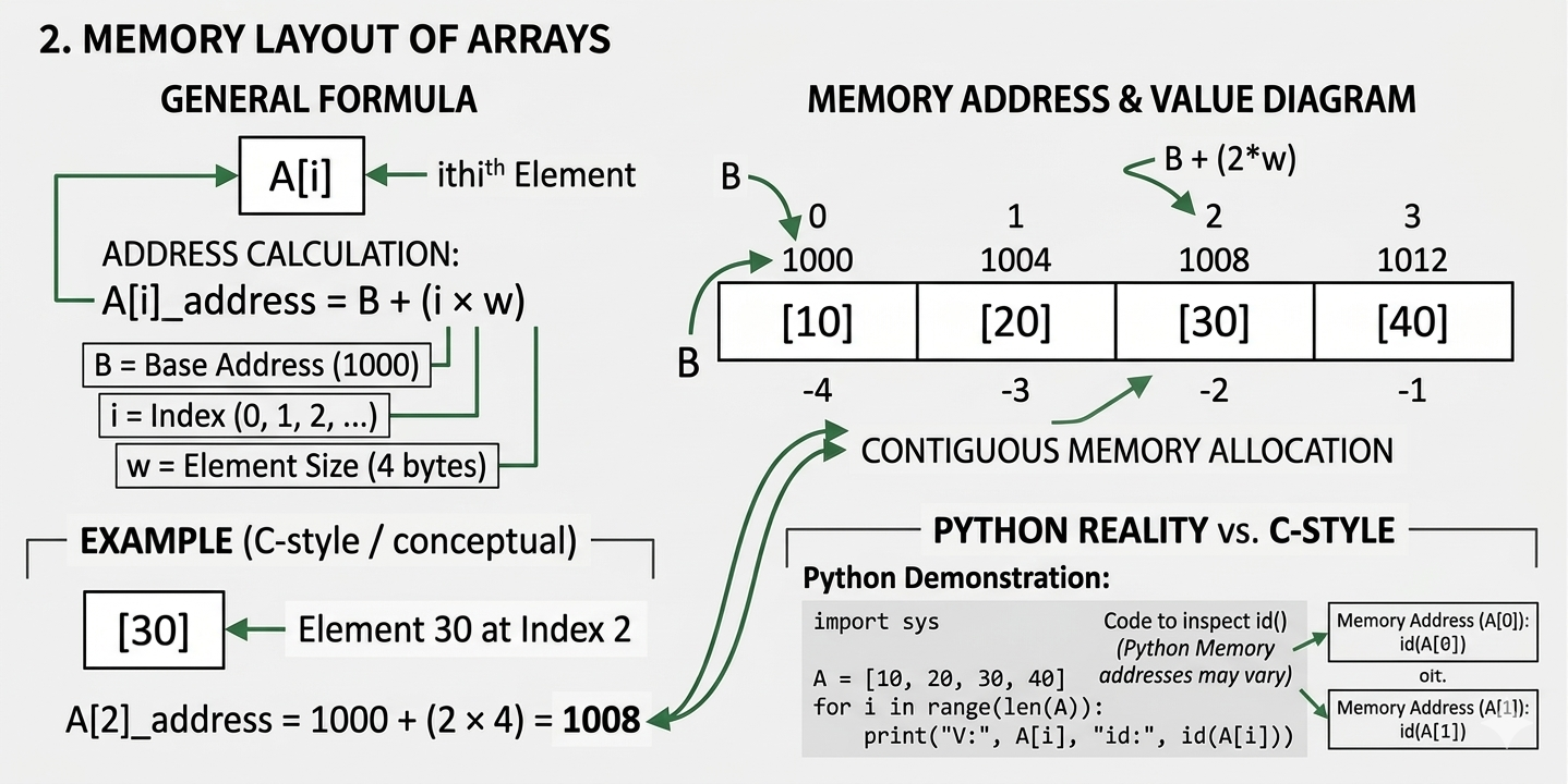
The defining property of arrays is contiguous memory allocation.

If the base address of the array is B and the size of each element is w bytes, then the address of the ith element is calculated using:

Where:

• B = base address
• i = index
• w = size of each element

Example

Suppose:

• Base address = 1000
• Element size = 4 bytes

A = [10, 20, 30, 40]

Memory layout:

Index	Value	Address
0	10	1000
1	20	1004
2	30	1008
3	40	1012

Python Demonstration (Memory Address)

Python does not guarantee strict contiguous storage like C arrays, but we can still inspect memory addresses.

import sys

A = [10, 20, 30, 40]

for i in range(len(A)):
    print("Value:", A[i], "Address:", id(A[i]))

This prints the memory location of each element.

Types of Arrays

Arrays can be categorized based on dimensions.

One-Dimensional Array

A simple linear list of elements.

Example:

[5, 9, 3, 7]

Memory structure:

|5|9|3|7|

Python Example

arr = [5, 9, 3, 7]

# printing elements
for element in arr:
    print(element)

Applications include:

• Storing lists
• Buffers
• Temporary data storage

Two-Dimensional Array

A matrix-like structure with rows and columns.

Example:

A = [
 [1,2,3],
 [4,5,6],
 [7,8,9]
]

Python Example

matrix = [
    [1,2,3],
    [4,5,6],
    [7,8,9]
]

print(matrix[0][1])  # Output: 2
print(matrix[2][2])  # Output: 9

Used in:

• Image processing
• Game boards
• Mathematical matrices

Row-Major Order

Elements stored row by row.

Memory layout:

1 2 3 4 5 6 7 8 9

Address formula:

Where n = number of columns.

Python Row Traversal Example

matrix = [
    [1,2,3],
    [4,5,6],
    [7,8,9]
]

for row in matrix:
    for element in row:
        print(element, end=" ")

Column-Major Order

Elements stored column by column. Used in languages like Fortran and MATLAB.

Address formula:

Where m = number of rows.

Python Column Traversal Example

matrix = [
    [1,2,3],
    [4,5,6],
    [7,8,9]
]

rows = len(matrix)
cols = len(matrix[0])

for j in range(cols):
    for i in range(rows):
        print(matrix[i][j], end=" ")

Basic Array Operations

Arrays support several important operations.

Access

Retrieving an element using its index.

A[3]

Python Example

A = [10,20,30,40]

print(A[3])  # Output: 40

Time complexity: O(1)

Traversal

Visiting each element in sequence.

A = [10,20,30,40]

for x in A:
    print(x)

Time complexity: O(n)

Insertion

Inserting into the middle requires shifting elements.

Example:

• Before: [10,20,30,40]
• Insert 25 at index 2
• After: [10,20,25,30,40]

Python Example

A = [10,20,30,40]

A.insert(2,25)

print(A)

Time complexity: O(n)

Deletion

Removing an element also requires shifting.

Example:

• Before: [10,20,30,40]
• Delete index 1
• After: [10,30,40]

Python Example

A = [10,20,30,40]

del A[1]

print(A)

Time complexity: O(n)

Static vs Dynamic Arrays

Static Arrays

Fixed size allocated at compile time.

Example in C:

int A[10];

Python Note

Python does not have static arrays by default, but the array module can simulate them.

import array

A = array.array('i', [1,2,3,4])
print(A)

Dynamic Arrays

Resizable arrays allocated during runtime.

Examples:

• Python lists
• C++ vectors
• Java ArrayList

Python Example

A = [1,2,3]

A.append(4)
A.append(5)

print(A)

Dynamic arrays automatically resize when capacity is exceeded.

Dynamic Array Resizing

When capacity is full:

1. Allocate larger array
2. Copy elements
3. Insert new element

This copying costs O(n), but the amortized cost of insertion remains O(1) because resizing happens rarely.

A = []

for i in range(10):
    A.append(i)

print(A)

Advantages of Arrays

Fast Access

Direct index access gives O(1) time.

Memory Efficiency

Contiguous memory improves cache performance.

Simplicity

Arrays are easy to implement and understand.

Limitations of Arrays

Fixed Size (Static Arrays)

Cannot grow automatically.

Costly Insertions and Deletions

Shifting elements causes O(n) time complexity.

Homogeneous Elements

All elements must be of the same data type in low-level languages.

Applications of Arrays

Arrays appear in numerous real-world systems.

Matrix Computations

Scientific computing relies heavily on arrays.

• Linear algebra
• Physics simulations

import numpy as np

matrix = np.array([[1,2],[3,4]])

print(matrix)

Image Processing

Images are stored as 2D arrays of pixels.

import numpy as np

image = np.zeros((5,5))

print(image)

Database Systems

Indexes and buffers often use arrays.

Sorting Algorithms

Many sorting algorithms operate directly on arrays.

• Merge sort
• Quick sort
• Heap sort

A = [5,3,8,1]

A.sort()

print(A)

Graph Algorithms

Graphs may be represented using adjacency matrices, which are arrays.

graph = [
    [0,1,0],
    [1,0,1],
    [0,1,0]
]

print(graph[0][1])  # edge between node 0 and 1

Arrays in Modern Programming Languages

Most programming languages implement arrays differently.

Language	Implementation
C	Fixed-size arrays
C++	Arrays & vectors
Java	Array objects
Python	Dynamic lists
JavaScript	Dynamic arrays

Despite differences, the core concept remains the same.

Time Complexity Summary

Operation	Time Complexity
Access	O(1)
Search	O(n)
Insertion	O(n)
Deletion	O(n)
Traversal	O(n)

Why Arrays Are So Important

Arrays are foundational because they:

• Provide fast random access
• Enable efficient memory usage
• Serve as the building blocks for complex data structures

Many advanced structures depend on arrays, including:

• Heaps
• Hash tables
• Dynamic programming tables
• Graph adjacency matrices

Understanding arrays deeply is essential for mastering data structures and algorithm design.

Common Array Methods in Python

In Python, arrays are commonly implemented using lists, which provide many built-in methods to manipulate data efficiently.

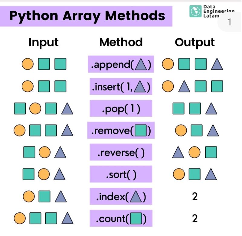
append()

The append() method adds an element to the end of the array.

Syntax

array.append(element)

Example

A = [10, 20, 30]

A.append(40)

print(A)

Output: [10, 20, 30, 40]

Time Complexity: O(1) (amortized)

insert()

The insert() method adds an element at a specific index.

Syntax

array.insert(index, element)

Example

A = [10, 20, 30, 40]

A.insert(2, 25)

print(A)

Output: [10, 20, 25, 30, 40]

Time Complexity: O(n) — because elements need to shift.

remove()

The remove() method deletes the first occurrence of a value.

Syntax

array.remove(value)

Example

A = [10, 20, 30, 20]

A.remove(20)

print(A)

Output: [10, 30, 20]

pop()

The pop() method removes and returns an element. If no index is given, it removes the last element.

Syntax

array.pop(index)

Example

A = [10, 20, 30, 40]

A.pop()

print(A)

Output: [10, 20, 30]

Example with index

A = [10, 20, 30, 40]

A.pop(1)

print(A)

Output: [10, 30, 40]

index()

The index() method returns the index of a value.

Syntax

array.index(value)

Example

A = [10, 20, 30, 40]

print(A.index(30))

Output: 2

count()

The count() method counts how many times an element appears.

Syntax

array.count(value)

Example

A = [10, 20, 20, 30]

print(A.count(20))

Output: 2

sort()

The sort() method sorts the array in ascending order.

Syntax

array.sort()

Example

A = [5, 2, 8, 1]

A.sort()

print(A)

Output: [1, 2, 5, 8]

Descending order:

A.sort(reverse=True)

reverse()

The reverse() method reverses the order of elements.

Syntax

array.reverse()

Example

A = [1, 2, 3, 4]

A.reverse()

print(A)

Output: [4, 3, 2, 1]

extend()

The extend() method adds elements from another array.

Syntax

array.extend(other_array)

Example

A = [1, 2, 3]
B = [4, 5, 6]

A.extend(B)

print(A)

Output: [1, 2, 3, 4, 5, 6]

clear()

The clear() method removes all elements from the array.

Syntax

array.clear()

Example

A = [10, 20, 30]

A.clear()

print(A)

Output: []

Conclusion

Arrays are one of the most essential data structures in computer science. Their contiguous memory layout enables constant-time access and efficient computation.

Although arrays have limitations such as costly insertions and fixed sizes in some languages, they remain a cornerstone of algorithm design and system implementation.

Mastering arrays and their memory structure is the first step toward understanding more advanced data structures.