Amortized Analysis

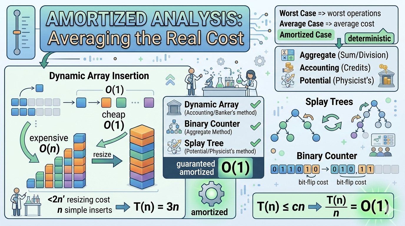
In algorithm analysis, some operations look expensive in isolation — but when averaged over many operations, they turn out to be efficient. That's where amortized analysis comes in.

Instead of analyzing the worst-case cost of a single operation, amortized analysis asks:

What is the average cost per operation over a sequence of operations?

It guarantees performance without using probability.

Why Amortized Analysis Is Needed

Consider a dynamic array (like Python lists or C++ vectors).

Most insertions take O(1). But occasionally, when the array is full, we must:

• Allocate new memory
• Copy all elements
• Insert the new element

That resizing step costs O(n). So is insertion O(n)?

No. Because resizing happens rarely. Amortized analysis shows insertion is still:

Worst Case vs Amortized vs Average Case

Type	Meaning
Worst Case	Maximum cost of one operation
Average Case	Expected cost over random inputs
Amortized	Guaranteed average per operation over a sequence

The Three Methods of Amortized Analysis

• Aggregate Method
• Accounting Method
• Potential Method

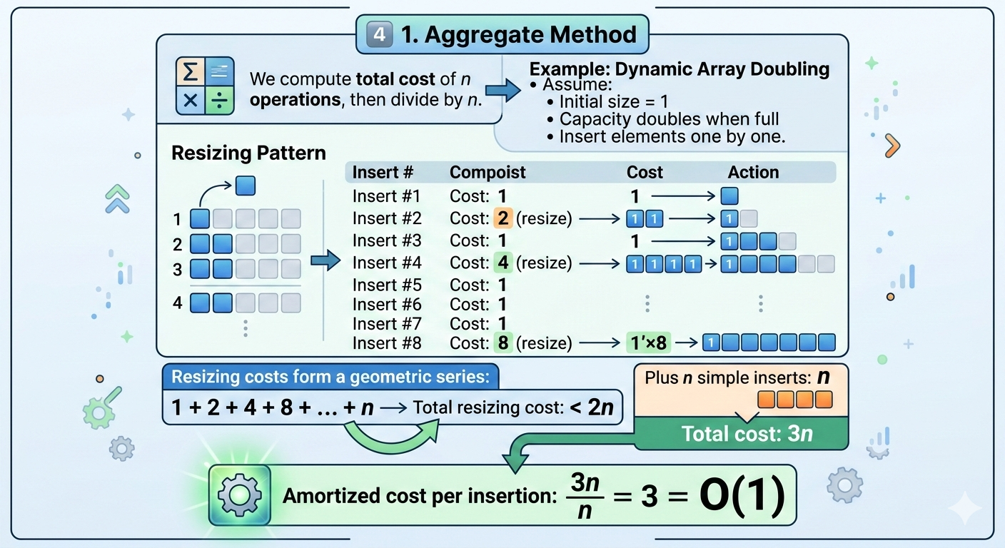
Aggregate Method

We compute the total cost of n operations, then divide by n.

Example: Dynamic Array Doubling

Assume initial size = 1 and capacity doubles when full. Insert elements one by one.

Resizing Pattern

Insert #	Cost
1	1
2	2 (resize)
3	1
4	4 (resize)
5	1
6	1
7	1
8	8 (resize)

Resizing costs form a geometric series:

Plus n simple inserts. Total cost:

Amortized cost per insertion:

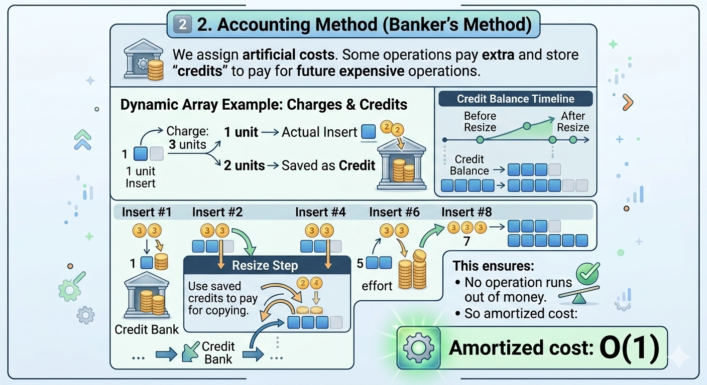
Accounting Method (Banker's Method)

We assign artificial costs. Some operations pay extra and store "credits" to pay for future expensive operations.

Dynamic Array Example

Charge 3 units per insertion:

• 1 unit → actual insert
• 2 units → saved as credit

When a resize happens, use the saved credits to pay for copying. This ensures no operation ever runs out of budget. So amortized cost:

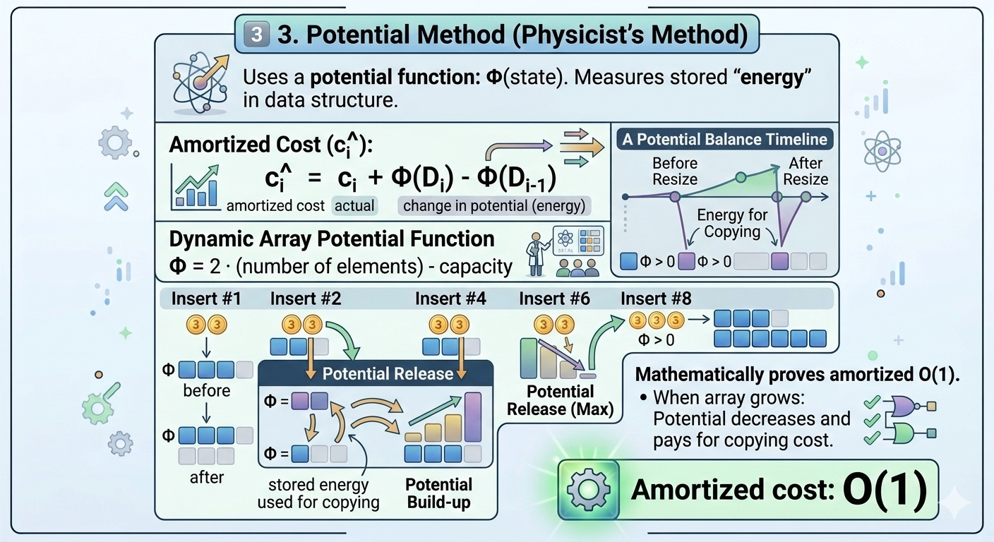
Potential Method (Physicist's Method)

Uses a potential function Φ(state) that measures stored "energy" in the data structure.

Amortized cost of the i-th operation:

Where cᵢ is the actual cost and Φ is the potential.

Dynamic Array Potential Function

Let:

When the array grows, potential decreases and pays for the copying cost — mathematically proving amortized O(1).

Stack with Multipop Operation

Operations:

• PUSH → O(1)
• POP → O(1)
• MULTIPOP(k) → up to O(k)

Worst case: MULTIPOP(n) = O(n).

But across a sequence, each element can be popped only once. So total pops ≤ total pushes. If we do n operations:

Amortized cost per operation:

Binary Counter Example

Incrementing a binary number:

0000 → 0001
0001 → 0010
0010 → 0011
0011 → 0100

Sometimes many bits flip. Worst-case increment: O(log n).

But over n increments, each bit flips at most n times divided by powers of 2. Total flips:

So amortized cost per increment:

Amortized Analysis of Splay Trees

Splay trees use rotations to self-organize. A single operation may cost O(n), but using the potential method:

Amortized vs Worst-Case Guarantees

Data Structure	Worst Case	Amortized
Dynamic Array Insert	O(n)	O(1)
Binary Counter	O(log n)	O(1)
Splay Tree	O(n)	O(log n)

Amortized guarantees are deterministic over a sequence — no randomness required.

When to Use Amortized Analysis

Used in:

• Dynamic arrays
• Hash tables resizing
• Garbage collection
• Network buffering
• Persistent data structures
• Functional programming structures

Why Amortized Analysis Works

Key principle: expensive operations are rare. If costly events happen infrequently enough, their cost spreads over many cheap operations, bringing the per-operation average down to a constant or logarithmic bound.

Common Mistakes

• Confusing amortized with average-case
• Forgetting to count the full sequence cost
• Not justifying the potential function
• Ignoring adversarial sequences

Mathematical Summary

If the total cost of n operations is:

Then the amortized cost per operation is:

Even if some individual operations cost O(n).

Real-World Impact

Amortized analysis explains why:

• Python lists scale well
• C++ vectors are efficient
• Databases resize indexes safely
• Memory allocators remain fast
• Web servers handle traffic spikes

Final Summary

Amortized analysis studies performance over sequences, not single operations.

Three main methods:

• Aggregate Method — sum total cost, divide by n
• Accounting Method — assign credits to cheap ops, spend on expensive ones
• Potential Method — use a potential function to track stored "energy"

It proves that some operations with bad worst-case behavior are still efficient overall — bridging the gap between theory and practical system design.