Randomized Algorithms Basics
Using Randomness to Design Efficient Algorithms
In classical algorithms, the output is completely determined by the input. However, randomized algorithms introduce randomness during execution to improve performance, simplify design, or handle difficult problems.
Randomized algorithms play a major role in modern computing, including:
- Cryptography
- Machine learning
- Distributed systems
- Databases
- Network routing
- Load balancing
In this article, we explore the fundamentals of randomized algorithms, their mathematical foundations, and how to analyze them.
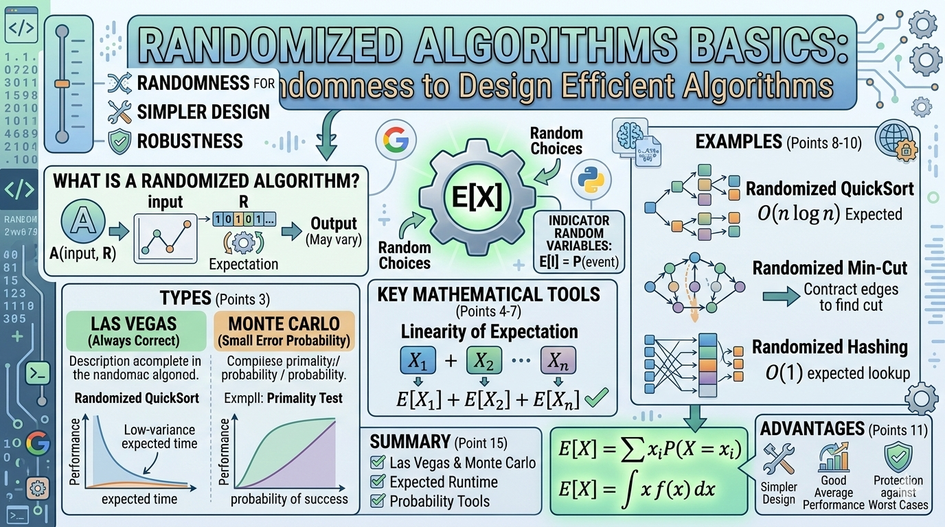
What is a Randomized Algorithm?
A randomized algorithm is an algorithm that makes random choices during its execution.
Because of these random choices:
- Running the algorithm twice on the same input may produce different execution paths
- The result may vary in performance or correctness probability
Formal Definition
A randomized algorithm uses a source of randomness R. The algorithm becomes:
Where:
- input = problem instance
- R = sequence of random bits
The performance is analyzed in expectation over R.
Why Use Randomized Algorithms?
Randomized algorithms are often:
1. Simpler
Some deterministic algorithms are very complex, but randomness simplifies them.
2. Faster
Randomized algorithms often achieve better expected running time.
3. Robust
They prevent adversarial inputs designed to break deterministic algorithms.
4. Widely Used
Examples include:
| Area | Randomized Algorithm |
|---|---|
| Sorting | Randomized QuickSort |
| Hashing | Universal Hashing |
| Graph Algorithms | Randomized Min-Cut |
| Cryptography | Randomized primality testing |
Types of Randomized Algorithms
Randomized algorithms fall into two major categories.
Las Vegas Algorithms
These algorithms:
- Always produce correct results
- Running time is random
Example
Randomized QuickSort. Output is always correct, but runtime varies depending on pivot choices.
Expected complexity:
Worst case:
But worst case happens with very low probability.
Monte Carlo Algorithms
These algorithms:
- Have fixed running time
- May produce incorrect answers with small probability
Example
Primality testing algorithm: It may say a composite number is prime with small probability. Error probability can be reduced by repeating the test.
Mathematical Tools for Randomized Algorithms
To analyze randomized algorithms we use probability theory.
Key concepts include:
- Expected value
- Indicator variables
- Linearity of expectation
- Probability bounds
Expected Value
Expected value measures the average outcome of a random variable.
Definition
If X is a random variable:
For continuous variables:
Example
Suppose an algorithm picks a random number from {1, 2, 3}. Expected value:
Expected value helps measure expected running time.
Indicator Random Variables
Indicator variables simplify probability analysis.
Define:
Expected value:
Indicator variables are widely used in algorithm analysis.
Linearity of Expectation
One of the most powerful tools.
Theorem
For random variables X₁, X₂, ..., Xₙ:
This holds even if variables are not independent. This makes algorithm analysis much easier.
Example: Randomized QuickSort
Randomized QuickSort chooses the pivot randomly.
Algorithm
- Pick random pivot
- Partition array
- Recursively sort subarrays
Expected Running Time
Worst case:
Expected time:
Random pivot selection ensures balanced partitions on average.
Example: Randomized Min-Cut (Karger's Algorithm)
Goal: Find the minimum cut in a graph.
Algorithm
- Randomly pick an edge
- Contract it
- Repeat until two nodes remain
The remaining edges form the cut.
Probability of finding minimum cut:
Repeating the algorithm many times increases success probability.
Randomized Hashing
Hash tables often use randomized functions.
Example
Where:
- a, b chosen randomly
- p is a prime
This technique prevents worst-case collisions. Expected lookup time:
Advantages of Randomized Algorithms
1. Simpler Design
Many randomized algorithms are easier to implement.
2. Good Average Performance
Often faster than deterministic algorithms.
3. Protection Against Worst Cases
Randomness prevents adversarial inputs.
Disadvantages
- Non-deterministic behavior — Two runs may differ
- Probability of error (Monte Carlo algorithms) — Results may occasionally be wrong
- Need for randomness source — Algorithms depend on good random number generators
Applications in Real Systems
Randomized algorithms power many real-world systems.
Examples include:
Google Search
Randomized hashing and sampling.
Load Balancing
Randomized request distribution.
Machine Learning
Stochastic gradient descent uses random sampling.
Cryptography
Random primes and random keys.
Derandomization
Sometimes we convert randomized algorithms into deterministic ones. This process is called derandomization.
Techniques include:
- Pseudorandom generators
- Method of conditional expectations
- Deterministic simulations
Derandomization is an active research area in theoretical computer science.
Summary
Randomized algorithms use randomness to improve algorithm performance and simplicity.
Key ideas include:
- Las Vegas algorithms (always correct)
- Monte Carlo algorithms (small probability of error)
- Expected running time analysis
- Indicator variables
- Linearity of expectation
Randomized techniques are widely used in modern computing and algorithm design.
Randomness is a powerful tool in algorithm design that often leads to simpler and faster algorithms.