Dynamic Arrays Implementation: How Resizable Arrays Work Internally

1. Introduction

Imagine you are developing a social media application where users can upload photos.

When a user creates an account, you don't know whether they will upload 5 photos, 100 photos, or 10,000 photos.

If you use a fixed-size array with space for 100 photos, two problems can occur:

• If the user uploads only 5 photos, most of the allocated memory remains unused.
• If the user uploads more than 100 photos, the array cannot accommodate additional elements without creating a new array.

This is where dynamic arrays become useful.

A dynamic array is a data structure that automatically adjusts its storage capacity as elements are added or removed. Unlike traditional fixed-size arrays, dynamic arrays allow us to manage collections whose sizes change during program execution.

Popular examples include:

• ArrayList in Java
• vector in C++
• List<T> in C#
• list in Python (implemented using a resizable array of references)

Although these structures appear simple from a programmer's perspective, they rely on important concepts such as memory allocation, element copying, resizing strategies, and amortized complexity.

In this article, we will explore how dynamic arrays work internally and implement one from scratch using Python.

2. Static Arrays vs Dynamic Arrays

Before understanding dynamic arrays, let's revisit static arrays.

Static Arrays

A static array has a fixed capacity determined when its storage is allocated.

int numbers[5] = {10, 20, 30, 40, 50};

This array can hold exactly five integers. Its elements are stored in contiguous memory locations.

Index:     0    1    2    3    4
         +----+----+----+----+----+
Values:  | 10 | 20 | 30 | 40 | 50 |
         +----+----+----+----+----+

Accessing an element is extremely efficient because its memory address can be calculated directly. However, increasing the capacity requires allocating different storage.

Dynamic Arrays

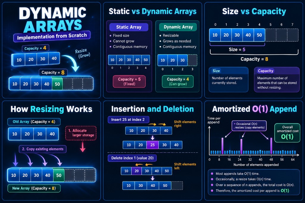
A dynamic array also uses contiguous storage, but its allocated capacity can change. Consider an array that initially has room for four elements:

Size = 3
Capacity = 4

         +----+----+----+-------+
Values:  | 10 | 20 | 30 | Empty |
         +----+----+----+-------+

After inserting another element:

Size = 4
Capacity = 4

         +----+----+----+----+
Values:  | 10 | 20 | 30 | 40 |
         +----+----+----+----+

Now suppose we want to insert 50. The array has reached its maximum capacity. Instead of rejecting the insertion, a dynamic array allocates a larger storage block and copies the existing elements into it.

Old Array (Capacity = 4)

+----+----+----+----+
| 10 | 20 | 30 | 40 |
+----+----+----+----+

           |
           | Allocate larger storage
           v

New Array (Capacity = 8)

+----+----+----+----+----+----+----+----+
| 10 | 20 | 30 | 40 | 50 |    |    |    |
+----+----+----+----+----+----+----+----+

Size = 5
Capacity = 8

This ability to grow automatically is the defining characteristic of a dynamic array.

Comparison

Feature	Static Array	Dynamic Array
Capacity	Fixed	Resizable
Memory layout	Contiguous	Contiguous
Random access	O(1)	O(1)
Append	O(1) if space exists	O(1) amortized
Insertion in middle	O(n)	O(n)
Memory overhead	Usually minimal	Extra reserved capacity
Flexibility	Limited	High

3. Understanding Size and Capacity

Two important properties determine how a dynamic array operates.

Size

The number of elements currently stored in the array.

Capacity

The maximum number of elements that can fit into the currently allocated storage without resizing.

+----+----+----+----+----+----+----+----+
|  5 | 10 | 15 | 20 |    |    |    |    |
+----+----+----+----+----+----+----+----+

Size = 4
Capacity = 8

Even though eight positions are allocated, only four contain valid elements. Therefore:

The number of unused slots is:

For our example:

Four additional elements can be appended without reallocating memory.

Why not allocate exactly the required size?

Suppose an array contains five elements and has a capacity of five. If every new insertion requires allocating an array with exactly one additional slot, the system must repeatedly:

1. Allocate a new array.
2. Copy all existing elements.
3. Insert the new element.
4. Release the old storage.

This creates significant overhead. Dynamic arrays solve this problem by allocating extra capacity in advance.

4. How Dynamic Array Resizing Works

One of the most common resizing strategies is geometric growth. When the array becomes full, its capacity is multiplied by a constant growth factor. For example, a doubling strategy uses:

where C represents capacity. Suppose the initial capacity is 2. The growth sequence becomes:

2 → 4 → 8 → 16 → 32 → 64 → ...

Let's observe how an array grows as we insert elements.

Insertion	Size	Capacity	Resize?
Insert 10	1	2	No
Insert 20	2	2	No
Insert 30	3	4	Yes
Insert 40	4	4	No
Insert 50	5	8	Yes
Insert 60	6	8	No
Insert 70	7	8	No
Insert 80	8	8	No
Insert 90	9	16	Yes

Notice something interesting: resizing does not happen during every insertion. It happens only when the array reaches its current capacity. This is why dynamic arrays achieve efficient average performance across long sequences of append operations.

Why doubling?

Doubling provides a useful trade-off between:

• The number of memory reallocations
• The number of elements copied
• The amount of unused allocated memory

A larger growth factor reduces resizing frequency but may waste more memory. A smaller growth factor saves space but causes more frequent reallocations.

Different programming languages and libraries use different growth policies. Doubling is a convenient strategy for understanding the underlying algorithm.

5. Implementing a Dynamic Array from Scratch in Python

Although Python already provides dynamic arrays through its built-in list, we will use the ctypes module to create fixed-capacity storage for Python object references. This allows us to simulate the important internal operations of a dynamic array.

Our implementation will support:

• Appending elements
• Accessing elements by index
• Updating elements
• Inserting elements at a specific position
• Removing elements
• Resizing the underlying storage
• Getting the current size and capacity

Step 1: Create the Class

import ctypes

class DynamicArray:
    def __init__(self):
        self.size = 0
        self.capacity = 1
        self.array = self._make_array(self.capacity)

    def _make_array(self, capacity):
        return (capacity * ctypes.py_object)()

• self.size tracks how many elements are currently stored.
• self.capacity tracks how many elements can be stored without resizing.
• self.array holds the underlying fixed-capacity storage.
• _make_array() creates a contiguous array of Python object references.

We start with a capacity of one.

Step 2: Implement Element Access

def __getitem__(self, index):
    if not 0 <= index < self.size:
        raise IndexError("Index out of range")

    return self.array[index]

This method allows us to access elements using normal indexing syntax such as arr[0]. Because the array uses contiguous storage, element access takes constant time:

The address of a slot can be calculated directly using the starting address and the slot's index.

Step 3: Implement Resizing

def _resize(self, new_capacity):
    new_array = self._make_array(new_capacity)

    for i in range(self.size):
        new_array[i] = self.array[i]

    self.array = new_array
    self.capacity = new_capacity

This is the most important method in our implementation. When resizing:

1. A new storage block is allocated.
2. Existing elements are copied into the new block.
3. The dynamic array switches to the new storage.
4. The old storage becomes eligible for reclamation when no references to it remain.

If the array currently contains n elements, copying them requires:

An individual resize has linear time complexity — but with geometric growth, resizing happens infrequently.

Step 4: Implement Append

def append(self, value):
    if self.size == self.capacity:
        self._resize(2 * self.capacity)

    self.array[self.size] = value
    self.size += 1

The append operation first checks whether the array has available space. If the array is full, its capacity is doubled before insertion.

arr = DynamicArray()

arr.append(10)
arr.append(20)
arr.append(30)

Internally:

Append 10:
[10]                 Size=1, Capacity=1

Append 20:
[10, 20]             Size=2, Capacity=2

Append 30:
[10, 20, 30, _]      Size=3, Capacity=4

The underscore represents unused capacity.

Step 5: Implement Insertion

Appending adds an element to the end. To insert at a specific position, we must shift the elements after that position one step to the right. Inserting 25 at index 2:

Before:
[10, 20, 30, 40, _]

After shifting:
[10, 20, _, 30, 40]

After insertion:
[10, 20, 25, 30, 40]

def insert(self, index, value):
    if not 0 <= index <= self.size:
        raise IndexError("Index out of range")

    if self.size == self.capacity:
        self._resize(2 * self.capacity)

    for i in range(self.size, index, -1):
        self.array[i] = self.array[i - 1]

    self.array[index] = value
    self.size += 1

In the worst case, inserting at the beginning requires shifting every existing element:

Step 6: Implement Deletion

Deleting an element from the middle requires shifting the remaining elements to the left.

Before:
[10, 20, 30, 40, 50]

Delete index 1:
[10, 30, 40, 50, _]

def remove_at(self, index):
    if not 0 <= index < self.size:
        raise IndexError("Index out of range")

    removed = self.array[index]

    for i in range(index, self.size - 1):
        self.array[i] = self.array[i + 1]

    self.size -= 1
    self.array[self.size] = None

    return removed

Setting the final unused slot to None releases the reference held by that slot. The worst-case time complexity is:

Notice that our implementation does not automatically shrink the array after deletion. We will discuss shrinking strategies later.

6. Complete Dynamic Array Implementation

Here is the complete working implementation combining all the methods.

import ctypes


class DynamicArray:
    def __init__(self):
        self.size = 0
        self.capacity = 1
        self.array = self._make_array(self.capacity)

    def _make_array(self, capacity):
        return (capacity * ctypes.py_object)()

    def __len__(self):
        return self.size

    def __getitem__(self, index):
        if not 0 <= index < self.size:
            raise IndexError("Index out of range")

        return self.array[index]

    def __setitem__(self, index, value):
        if not 0 <= index < self.size:
            raise IndexError("Index out of range")

        self.array[index] = value

    def _resize(self, new_capacity):
        new_array = self._make_array(new_capacity)

        for i in range(self.size):
            new_array[i] = self.array[i]

        self.array = new_array
        self.capacity = new_capacity

    def append(self, value):
        if self.size == self.capacity:
            self._resize(2 * self.capacity)

        self.array[self.size] = value
        self.size += 1

    def insert(self, index, value):
        if not 0 <= index <= self.size:
            raise IndexError("Index out of range")

        if self.size == self.capacity:
            self._resize(2 * self.capacity)

        for i in range(self.size, index, -1):
            self.array[i] = self.array[i - 1]

        self.array[index] = value
        self.size += 1

    def remove_at(self, index):
        if not 0 <= index < self.size:
            raise IndexError("Index out of range")

        removed = self.array[index]

        for i in range(index, self.size - 1):
            self.array[i] = self.array[i + 1]

        self.size -= 1
        self.array[self.size] = None

        return removed

    def pop(self):
        if self.size == 0:
            raise IndexError("Pop from empty array")

        return self.remove_at(self.size - 1)

    def __repr__(self):
        values = [
            repr(self.array[i])
            for i in range(self.size)
        ]

        return "[" + ", ".join(values) + "]"


# Example usage

arr = DynamicArray()

arr.append(10)
arr.append(20)
arr.append(30)

print("Initial:", arr)

arr.insert(1, 15)
print("After insertion:", arr)

arr.remove_at(2)
print("After deletion:", arr)

arr[0] = 100
print("After update:", arr)

print("Size:", len(arr))
print("Capacity:", arr.capacity)

Output:

Initial: [10, 20, 30]
After insertion: [10, 15, 20, 30]
After deletion: [10, 15, 30]
After update: [100, 15, 30]
Size: 3
Capacity: 4

Our custom dynamic array now supports the fundamental operations found in many production programming languages. This is an educational implementation rather than a replacement for Python's built-in list, which is implemented in optimized native code and supports many additional features.

7. Time Complexity Analysis

Operation	Best / Typical Case	Worst Case
Access by index	O(1)	O(1)
Update by index	O(1)	O(1)
Append	O(1)	O(n)
Pop from end	O(1)	O(1)
Insert at beginning	O(n)	O(n)
Insert at middle	O(n)	O(n)
Delete at beginning	O(n)	O(n)
Delete at middle	O(n)	O(n)
Resize	O(n)	O(n)

Appending an element normally takes O(1), but when resizing is necessary, it takes O(n). So why do we say that appending to a dynamic array has O(1) amortized complexity? Let's explore.

8. Amortized Analysis: Why Append Is O(1)

Suppose we start with a dynamic array of capacity one and repeatedly append elements. Using a doubling strategy, resizing occurs when the capacity grows:

1 → 2 → 4 → 8 → 16 → ...

Each resize copies the elements already present in the array. If we append n elements, the total number of elements copied across all resizing operations is bounded by a geometric series:

The total cost of copying is therefore O(n). Inserting the n new elements also requires O(n). Combining both costs:

Now divide the total cost by the number of append operations:

What does amortized mean?

Amortized analysis examines the average cost per operation over a sequence of operations, including occasional expensive operations. It does not mean that every append takes constant time — some appends trigger an expensive resize. However, those expensive operations happen rarely enough that the total cost remains linear over a sequence of n appends.

This guarantee does not depend on random inputs or probability.

9. What Happens If We Increase Capacity by One?

Now consider a different resizing strategy: instead of doubling the capacity, we increase it by exactly one whenever the array becomes full.

1 → 2 → 3 → 4 → 5 → 6 → ...

Each time we append an element to a full array, we must copy all existing elements. For n insertions, the total copying cost becomes:

Therefore:

The amortized insertion cost becomes:

This is significantly worse than geometric growth.

Comparison

Growth Strategy	Total Cost of n Appends	Amortized Append
Increase by 1	O(n²)	O(n)
Multiply capacity by 1.5	O(n)	O(1)
Double capacity	O(n)	O(1)

For any fixed growth factor greater than one, geometric growth provides amortized constant-time append operations.

The strategy used to manage memory can dramatically change the performance of a data structure.

10. Space Complexity and Memory Overhead

Dynamic arrays use additional memory to support future insertions. Suppose an array contains five elements but has a capacity of eight.

+----+----+----+----+----+----+----+----+
| 10 | 20 | 30 | 40 | 50 |    |    |    |
+----+----+----+----+----+----+----+----+

Used slots:   5
Unused slots: 3
Total slots:  8

The space utilization can be calculated as:

For this example:

The remaining 37.5% is reserved capacity.

Space Complexity

For an array containing n elements, geometric growth requires:

With a doubling strategy, immediately after a resize the array may have substantial unused capacity. However, its allocated capacity remains proportional to the number of stored elements.

During resizing, both the old and new storage blocks may temporarily exist simultaneously. This temporarily increases memory consumption, although the asymptotic space complexity remains O(n).

In our Python implementation, the underlying array stores references to Python objects, not necessarily the objects themselves. Therefore, the actual memory consumption also depends on the objects being referenced.

11. Should Dynamic Arrays Shrink Automatically?

So far, our dynamic array only grows. But consider a dynamic array that expands to a capacity of 1024 elements, after which 1000 elements are removed:

Size = 24
Capacity = 1024

Most of the allocated storage is unused. One possible strategy is to reduce the capacity when utilization becomes sufficiently low:

Why not shrink at 50%?

Suppose an array has a capacity of eight and contains four elements. If we shrink immediately to a capacity of four, appending one element would trigger another resize to eight. Removing that element might trigger shrinking again.

Capacity 8 → 4 → 8 → 4 → 8

Repeated expansion and contraction can cause unnecessary memory allocations and copying. This problem is known as resizing thrashing. Using separate thresholds for growing and shrinking helps avoid it:

• Grow when the array is full.
• Shrink when utilization drops to 25%.
• Keep a minimum capacity of one.

This technique is an example of hysteresis in resource management.

Optional Shrinking Implementation

We can extend our remove_at() method with the following logic after clearing the unused slot:

if (
    self.capacity > 1
    and self.size <= self.capacity // 4
):
    new_capacity = max(1, self.capacity // 2)
    self._resize(new_capacity)

This allows the array to reclaim unused storage. However, deletion can now occasionally trigger an O(n) resize. With the quarter-full shrinking threshold and doubling growth policy, append and end-pop operations still have O(1) amortized complexity.

12. Dynamic Arrays vs Linked Lists

Dynamic arrays and linked lists are both commonly used to store collections of elements, but they organize memory differently. A dynamic array stores elements in contiguous slots; a linked list stores elements in nodes connected through references or pointers.

Dynamic Array

+----+----+----+----+
| 10 | 20 | 30 | 40 |
+----+----+----+----+

Linked List

[10 | next] → [20 | next] → [30 | next] → [40 | null]

Comparison

Operation	Dynamic Array	Singly Linked List
Access by index	O(1)	O(n)
Append	O(1) amortized	O(1) with tail pointer
Insert at beginning	O(n)	O(1)
Delete at beginning	O(n)	O(1)
Insert after known node	O(n) generally	O(1)
Memory locality	Excellent	Usually weaker
Extra memory	Reserved capacity	Pointer per node

Dynamic arrays often perform well in practice because contiguous storage improves cache locality. Modern processors retrieve memory in cache lines, so accessing one element can bring neighboring elements into the CPU cache. Linked lists generally have weaker spatial locality because their nodes may be scattered throughout memory.

This is one reason dynamic arrays are frequently preferred for general-purpose collections.

13. Real-World Applications of Dynamic Arrays

1. Social Media Feeds

Applications maintain collections of posts, comments, reactions, and other items. Resizable arrays are useful when the number of elements is not known in advance.

2. Game Development

Games frequently manage changing collections of entities, particles, and events. Dynamic arrays provide efficient iteration and fast indexed access.

3. Graph Algorithms

Adjacency lists are often implemented using dynamic arrays:

graph = [
    [1, 2],
    [0, 3],
    [0, 3],
    [1, 2]
]

Each inner list can grow as edges are added.

4. Database and Search Systems

Dynamic arrays can be used in temporary buffers, intermediate query results, and in-memory collections.

5. Machine Learning and Data Processing

Resizable collections are useful while gathering samples, recording results, or preparing data before converting it into fixed-size numerical arrays. For heavy numerical computation, specialized structures such as NumPy arrays are often more memory-efficient than Python lists.

14. Common Mistakes When Implementing Dynamic Arrays

Mistake 1: Confusing size with capacity

Size represents the number of valid elements, while capacity represents allocated storage. Accessing an unused slot should not be treated as accessing a valid element.

Mistake 2: Resizing after every insertion

Increasing capacity by one creates quadratic total insertion cost. Use geometric growth instead.

Mistake 3: Forgetting to copy existing elements

When allocating new storage, the existing elements must be preserved. Otherwise, resizing results in data loss.

Mistake 4: Shifting elements in the wrong direction

During insertion, elements should be shifted from right to left in terms of processing order. Otherwise, existing values may be overwritten before they can be moved.

Mistake 5: Keeping unnecessary references after deletion

In reference-based implementations, unused slots should be cleared when appropriate. Otherwise, objects may remain referenced unnecessarily.

Mistake 6: Assuming every append takes O(1) worst-case time

Appending has O(1) amortized complexity, but a resize can make an individual append O(n).

15. Interview Questions

Q1. Why is accessing an element in a dynamic array O(1)?

Because the underlying storage is contiguous and the address of a slot can be calculated directly from its index.

Q2. Why is appending O(1) amortized instead of O(1) worst case?

Most appends require only one insertion, but some trigger resizing and copying of all existing elements.

Q3. Why do dynamic arrays use geometric growth?

Geometric growth reduces the frequency of resizing and ensures O(1) amortized append complexity.

Q4. What happens when a dynamic array reaches full capacity?

It allocates larger storage, copies existing elements, updates its internal storage reference, and inserts the new element.

Q5. Why is insertion at the beginning O(n)?

Every existing element must be shifted one position to the right.

Q6. Does a dynamic array always use less memory than a linked list?

Not necessarily. Dynamic arrays reserve unused capacity, while linked lists store additional pointers for their nodes. Actual memory consumption depends on the implementation and workload.

Q7. Can a dynamic array resize without moving its elements?

Sometimes, a memory allocator may be able to extend an allocation in place. However, a dynamic array cannot generally rely on that possibility.

Q8. Is Python's list implemented using a linked list?

No. In CPython, lists use a resizable contiguous array of object references.

16. Practice Problems

Try implementing the following features without using Python's built-in list methods for the underlying dynamic array operations.

Problem 1 — Search Operation (Easy)

def find(self, value):
    pass

Return the index of the first occurrence of a value, or -1 if it does not exist. Target complexity: O(n).

Problem 2 — Reverse an Array (Easy)

def reverse(self):
    pass

Reverse the array in place without allocating another array. Target complexity: O(n) time and O(1) auxiliary space.

Problem 3 — Extend Operation (Medium)

def extend(self, iterable):
    pass

Append all elements from an iterable while maintaining efficient resizing behavior.

Problem 4 — Automatic Shrinking (Medium)

Modify the array to shrink its capacity when utilization falls below a chosen threshold. Explain why your threshold avoids repeated resizing.

Problem 5 — Growth Strategy Benchmark (Advanced)

Compare three growth strategies:

• Increase capacity by one.
• Increase capacity by a factor of 1.5.
• Double capacity.

Measure the number of reallocations, copied elements, and execution time for increasingly large inputs. Explain your observations using amortized analysis.

17. Key Takeaways

Dynamic arrays are one of the most widely used data structures because they combine the advantages of contiguous memory with flexible storage capacity.

1. Dynamic arrays are resizable arrays. They can increase their capacity as more elements are inserted.
2. Size and capacity are different. Size counts stored elements; capacity represents allocated slots.
3. Resizing requires additional work. Allocating new storage and copying elements takes O(n) time.
4. Geometric growth is essential for efficiency. It allows O(1) amortized append operations.
5. Random access remains O(1). Elements can be accessed directly using their indices.
6. Middle insertions and deletions take O(n). Elements must be shifted to preserve order.
7. Dynamic arrays trade extra memory for performance. Reserved capacity reduces the frequency of reallocations.

Final Thoughts

A dynamic array may look like a simple collection that automatically grows, but its internal design demonstrates several fundamental ideas in computer science. It shows how memory allocation strategies influence algorithm performance, why amortized analysis matters, and how a carefully designed data structure can provide efficient operations even when some individual operations are expensive.

Understanding dynamic arrays also prepares us for more advanced data structures such as stacks, queues, heaps, and hash tables. The next time you write:

numbers.append(42)

remember that this simple operation is supported by a carefully designed memory management strategy.

References and Further Reading

1. Cormen, T. H., Leiserson, C. E., Rivest, R. L., and Stein, C. — Introduction to Algorithms, 4th Edition. MIT Press.
2. Goodrich, M. T., Tamassia, R., and Goldwasser, M. H. — Data Structures and Algorithms in Python. Wiley.
3. Python Documentation — Data Structures
4. Python Documentation — ctypes
5. CPython Source Code — listobject.c

DSA Series — From Foundations to Advanced Problem Solving · Article 14 of the complete Data Structures & Algorithms learning journey.