Proof Techniques for Algorithms

Writing an algorithm is only half the job. In computer science, we must prove that an algorithm produces correct results, terminates, meets its time and space guarantees, and is optimal when applicable.

Proof techniques form the mathematical backbone of algorithm design. This article covers the most important proof methods used in algorithm analysis.

Why Proofs Matter

Without proofs, bugs may hide in edge cases, algorithms may fail for large inputs, performance claims may be incorrect, and systems may break under stress.

Proofs ensure:

• ✔ Reliability
• ✔ Scalability
• ✔ Mathematical rigor
• ✔ Trust in large systems

What Do We Prove About Algorithms?

There are four main properties we prove:

• Correctness — the algorithm produces the right output for all valid inputs
• Termination — the algorithm always stops
• Time / Space Complexity — resource usage stays within bounds
• Optimality — no algorithm can do better asymptotically

Proof by Mathematical Induction

Induction is the most common proof method for algorithms. It mirrors recursion directly — if you can prove correctness for the base case and show the inductive step holds, correctness follows for all inputs.

Structure of Induction

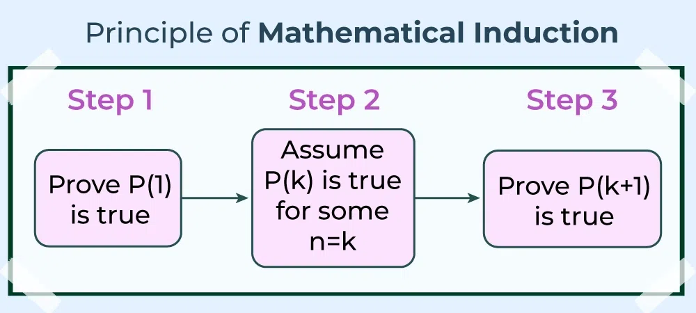
To prove a statement P(n):

1. Base Case — prove true for the smallest value
2. Inductive Hypothesis — assume true for n = k
3. Inductive Step — prove true for n = k + 1

If all three hold, the statement is true for all n.

Example: Sum of First n Numbers

Claim:

Base Case (n = 1): 1 = 1(2)/2 = 1 ✓

Inductive Step: Assume true for k:

For k + 1:

Thus proven. Recursive algorithms like factorial are typically verified this way.

Proof by Loop Invariant

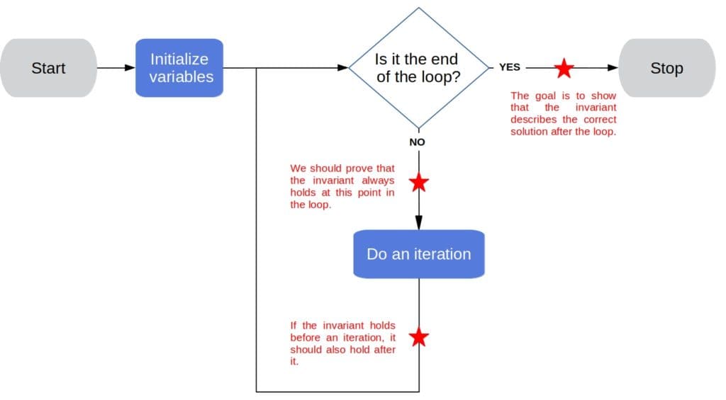
Loop invariants are used to prove correctness of iterative algorithms. A loop invariant is a property that is true before the loop starts and remains true after each iteration, enabling us to conclude correctness when the loop terminates.

Three Proof Steps

1. Initialization — the invariant holds before the first iteration
2. Maintenance — if the invariant holds before an iteration, it holds after
3. Termination — when the loop ends, the invariant gives us correctness

Example: Insertion Sort

Key invariant: at the start of each iteration, the first k elements are sorted.

• Initialization — a single element is trivially sorted
• Maintenance — inserting the next element into the correct position preserves order
• Termination — after n iterations, the entire array is sorted

Proof by Contradiction

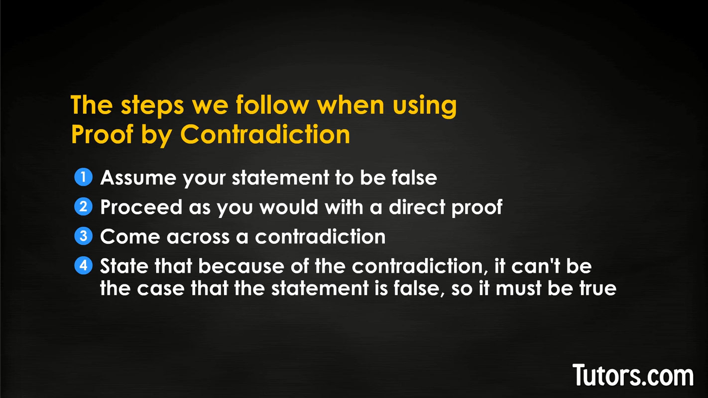
Used heavily in greedy algorithm proofs and lower bound arguments. The structure is simple: assume the opposite of what you want to prove, derive a logical contradiction, and conclude the original statement must be true.

Example: Greedy Choice Property

To prove a greedy algorithm is optimal:

1. Assume there exists a better solution OPT that differs from the greedy solution G
2. Modify OPT step-by-step to match greedy choices
3. Show each modification does not worsen the solution
4. Conclude OPT = G — contradiction with the assumption that a better solution exists

Common applications:

• Minimum Spanning Tree correctness (Kruskal's, Prim's)
• Shortest path proofs (Dijkstra's)
• Interval scheduling optimality

Proof by Contrapositive

Instead of proving A ⇒ B directly, prove its logical equivalent:

This is often easier when the contrapositive has a more natural structure. The two statements are logically identical — proving one proves the other.

Proof by Case Analysis

Break the problem into an exhaustive, mutually exclusive set of cases, and prove the statement holds in each. No case may be left uncovered.

Common uses in algorithms:

• Proving correctness of the absolute value function
• Binary search — three cases: target found, search left, search right
• Any algorithm with conditional branches

Proof of Termination

To prove an algorithm always terminates, identify a measure — a non-negative integer quantity — that strictly decreases after each step and cannot decrease below zero indefinitely.

while n > 0:
    n = n - 1

Here n decreases by 1 each iteration and cannot go below 0, so the loop always terminates in exactly n steps.

For recursive functions: ensure the argument passed to each recursive call is strictly smaller (closer to the base case) than the current argument.

Proof of Time Complexity

Time complexity proofs typically use one or more of:

• Recurrence relations — express runtime in terms of subproblem runtimes
• Asymptotic bounds — Big-O, Big-Theta, Big-Omega
• Induction — directly prove the closed-form bound

Example: Proving Merge Sort is O(n log n)

This can be solved by:

• Recursion tree — n work at each of log n levels → O(n log n)
• Master Theorem Case 2 — f(n) = n = Θ(n^log₂2) → O(n log n)
• Induction — assume T(n/2) ≤ c(n/2)log(n/2), substitute and simplify

Proof of Optimality

To show an algorithm is the best possible, we prove a lower bound — no algorithm, even undiscovered, can do better asymptotically.

Example: Comparison-Based Sorting Lower Bound

Claim: no comparison-based sorting algorithm can run faster than Ω(n log n).

1. Represent the algorithm's comparisons as a decision tree
2. The tree must have at least n! leaves (one per permutation)
3. A binary tree with n! leaves has height ≥ log(n!)
4. By Stirling's approximation: log(n!) = Ω(n log n)

Therefore no comparison-based sort can beat Ω(n log n) — making Merge Sort and Heap Sort asymptotically optimal.

Exchange Argument

A specialized technique for proving greedy algorithms are optimal. The idea: if an optimal solution differs from the greedy solution, we can exchange elements to match greedy choices one step at a time, without worsening the solution. After all exchanges, the greedy solution is shown to be equally optimal.

Used in:

• Activity selection problem
• Huffman coding
• Minimum spanning tree algorithms

Structural Induction

An extension of mathematical induction for recursive data structures like trees and lists. Instead of inducting on a number, we induct on the structure of the data.

Example: Proving a property of binary trees

1. Base case — prove the property holds for an empty tree (or a leaf)
2. Inductive hypothesis — assume it holds for the left and right subtrees
3. Inductive step — prove it holds for the full tree built from those subtrees

Common uses: binary tree traversal correctness, AVL tree height bounds, heap property proofs.

Amortized Analysis

Some operations are expensive occasionally but cheap on average. Amortized analysis proves that the average cost per operation over a sequence of operations is low, even if individual operations sometimes spike.

Example: Dynamic Array (ArrayList)

When appending to a full array, we double its size — costing O(n). But this happens rarely. Over n insertions:

• Resize costs: 1 + 2 + 4 + ⋯ + n = O(n) total
• Amortized cost per insertion: O(n) / n = O(1)

Proof methods:

• Aggregate analysis — total cost ÷ operations
• Accounting method — assign credits to cheap operations to pay for expensive ones
• Potential method — use a potential function to track stored energy

Common Algorithm Proof Patterns

Technique	Used For
Mathematical Induction	Recursive algorithms
Loop Invariant	Iterative correctness
Contradiction	Greedy optimality, lower bounds
Case Analysis	Conditional logic correctness
Recurrence Solving	Time complexity bounds
Amortized Analysis	Data structure average cost

Common Mistakes in Algorithm Proofs

• ❌ Forgetting the base case — induction without a starting point proves nothing
• ❌ Not proving termination — correctness is meaningless if the algorithm runs forever
• ❌ Circular reasoning — assuming what must be proven in the proof itself
• ❌ Ignoring edge cases — empty input, single element, maximum values
• ❌ Proving one example — a specific case does not constitute a general proof

Real-World Importance

Proof techniques are critical in domains where correctness is non-negotiable:

• Cryptography — security proofs rely on reduction arguments and lower bounds
• Operating systems — scheduler correctness, deadlock freedom
• Distributed systems — consensus algorithm correctness (Paxos, Raft)
• Database engines — transaction isolation and consistency proofs
• Safety-critical software — aviation, medical devices, nuclear control
• AI algorithms — convergence proofs for optimization methods

Major systems like compilers and encryption protocols are built on formal proofs verified by theorem provers. A bug in these systems can have catastrophic consequences — proofs replace hope with certainty.

Final Summary

Proof techniques are not academic formality — they are the engineering foundation of reliable algorithm design. They ensure:

• ✔ Correctness
• ✔ Termination
• ✔ Efficiency
• ✔ Optimality

Algorithms without proofs are guesses. Algorithms with proofs are engineering.