Space Complexity & Memory Models

Introduction

When analyzing algorithms, most beginners focus only on time complexity.

But in real systems, memory is just as important.

A fast algorithm that consumes excessive memory can:

• Crash systems
• Increase infrastructure cost
• Reduce scalability
• Cause cache inefficiency

Space complexity measures how much memory an algorithm uses relative to input size n.

Understanding memory behavior is critical for writing scalable and production-ready software.

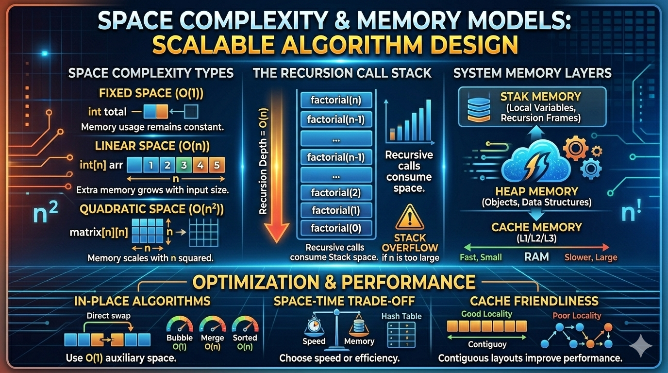
What Is Space Complexity?

Space complexity refers to the total memory required by an algorithm as a function of input size n.

It includes:

• Input space – memory required to store the input
• Auxiliary space – extra memory used by the algorithm

Types of Memory Usage

Fixed (Constant) Space

Memory usage does not grow with input size.

Example:

def sum_array(arr):
    total = 0
    for num in arr:
        total += num
    return total

Memory used:

• total → constant
• loop variable → constant

Space Complexity: O(1)

Even though time is O(n), space remains constant.

Linear Space

Memory grows proportionally with input size.

Example:

def copy_array(arr):
    new_arr = []
    for num in arr:
        new_arr.append(num)
    return new_arr

• If input size = n
• New array also size n

Space Complexity: O(n)

Quadratic Space

Memory grows as square of input size.

Example:

matrix = [[0 for _ in range(n)] for _ in range(n)]

This creates an n × n matrix.

Space Complexity: O(n²)

Recursive Space Complexity (Call Stack)

Recursion consumes memory via the call stack.

Each recursive call stores:

• Parameters
• Local variables
• Return address

Example: Linear Recursion

def factorial(n):
    if n == 0:
        return 1
    return n * factorial(n - 1)

• Depth of recursion = n
• Each call uses constant space

Total Space: O(n)

Example: Binary Recursion

def fibonacci(n):
    if n <= 1:
        return n
    return fibonacci(n-1) + fibonacci(n-2)

Although time is exponential, maximum recursion depth is n.

So space complexity: O(n)

In Place Algorithms

An algorithm is in-place if it uses O(1) extra memory.

Example: Swapping elements in an array

arr[i], arr[j] = arr[j], arr[i]

Sorting algorithms comparison:

Algorithm	Space Complexity
Merge Sort	O(n)
Quick Sort	O(log n) average
Bubble Sort	O(1)

In place algorithms are important for large datasets.

Space Complexity in Data Structures

Different data structures have different memory costs.

Arrays

• Contiguous memory
• Minimal overhead
• O(n) space

Linked Lists

Each node stores:

• Data
• Pointer

Extra pointer memory increases total usage.

Still: O(n)

But constant factor is larger than arrays.

Hash Tables

Require:

• Buckets
• Possible resizing
• Load factor management

Space: O(n)

But often larger memory footprint than arrays.

Trees

• Binary tree with n nodes: O(n)
• Balanced tree height: O(log n)
• Unbalanced tree height: O(n)

Memory structure affects performance.

Memory Models in Computer Systems

Understanding algorithm space requires understanding how memory works.

Stack Memory

Used for:

• Function calls
• Local variables
• Recursion frames

Characteristics:

• Fast allocation
• Automatically managed
• Limited size

Stack overflow occurs if recursion is too deep.

Heap Memory

Used for:

• Dynamic allocation
• Objects
• Data structures

Characteristics:

• Larger than stack
• Slower allocation
• Requires garbage collection or manual freeing

Example (Python automatically manages heap):

arr = [1, 2, 3]

Static / Global Memory

Stores:

• Global variables
• Static variables

Allocated once during program lifetime.

Cache and Memory Hierarchy

Modern systems have multiple memory layers:

• CPU Registers (fastest)
• L1 / L2 / L3 Cache
• RAM
• Disk

Memory access speed decreases dramatically down the hierarchy.

Example:

• Array traversal → cache friendly
• Linked list traversal → poor locality

Space layout affects performance.

Trade Off: Time vs Space

Sometimes we trade memory for speed.

Example:

Without extra memory:

• Search in array → O(n)

With hash table:

• Search → O(1) average
• But space increases to O(n)

This is called a: Space Time Tradeoff

Common in:

• Dynamic Programming (memoization)
• Caching
• Preprocessing tables

Space Complexity in Dynamic Programming

Example: Fibonacci

Recursive (no memoization):

• Time: O(2ⁿ)
• Space: O(n)

With memoization:

• Time: O(n)
• Space: O(n)

We used extra memory to reduce time.

Memory Optimization Techniques

• Use in place algorithms
• Avoid unnecessary copies
• Use iterative solutions instead of deep recursion
• Reuse variables
• Compress data when possible
• Use bit manipulation for compact storage

Real World Impact

Memory inefficiency causes:

• Application crashes
• Cloud cost increase
• Slow garbage collection
• Poor scalability
• Mobile app battery drain

Comparing Time vs Space Complexity

Scenario	Time	Space
Linear search	O(n)	O(1)
Merge sort	O(n log n)	O(n)
Quick sort	O(n log n)	O(log n)
Hash lookup	O(1)	O(n)

Good engineers optimize both dimensions.

Key Takeaways

• Space complexity measures memory growth.
• Focus on auxiliary space.
• Recursion consumes stack memory.
• In-place algorithms use O(1) space.
• Memory models (stack vs heap) affect performance.
• Cache locality matters in real systems.
• Space-time tradeoffs are fundamental in algorithm design.